Train a network, then look inside it

Every MNIST tutorial ends the same way: you get a number, somewhere around 97%, and a sentence congratulating you. Then it stops. Which is a shame, because the accuracy number is the one output of the exercise that teaches you nothing — it's a summary statistic of a thing you still haven't looked at.

The interesting part starts after training, when you load the weights and discover that one neuron out of 128 taught itself to detect a diagonal stroke and nobody told it to.

Here's the afternoon version, with the figures from my own run. Everything below is in github.com/silouone/mnist-anatomy — clone it, train it, and you'll get your own numbers in about 82 seconds.

Why this specific toy is worth your time

Handwritten digits are the right sandbox for one reason: the whole thing is small enough to print. 784 inputs, two hidden layers of 128 and 64, ten outputs. 109,386 trainable parameters — a number you can hold in your head, against the hundreds of billions in the models you actually use at work. The dataset is 11 MB. Training takes 82 seconds on a laptop. There is nowhere for mystery to hide.

That's the point. You cannot inspect a frontier model. You can inspect this one completely, and the mechanisms are the same ones, just fewer of them.

1 · Look at what actually goes in

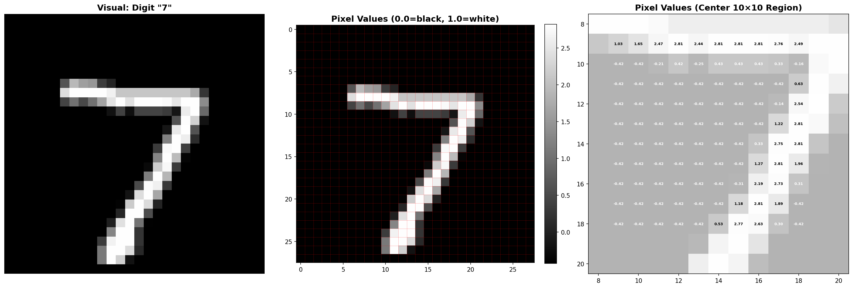
A handwritten 7 from MNIST shown as a 28×28 image beside its grid of raw pixel values between 0 and 1. — One MNIST digit, as the network receives it: 784 greyscale values.

Before anything else, print the input. A 28×28 image is 784 numbers between 0 and 1. That's the entire thing the network ever sees — no edges, no strokes, no "seven". Just a flat list of brightnesses, in a fixed order.

This is worth doing by hand once, because it's the same fact that governs the large models: everything is numbers before it reaches the network, and any structure you think is in there is structure the network will have to reconstruct for itself.

2 · Watch the gap open while it trains

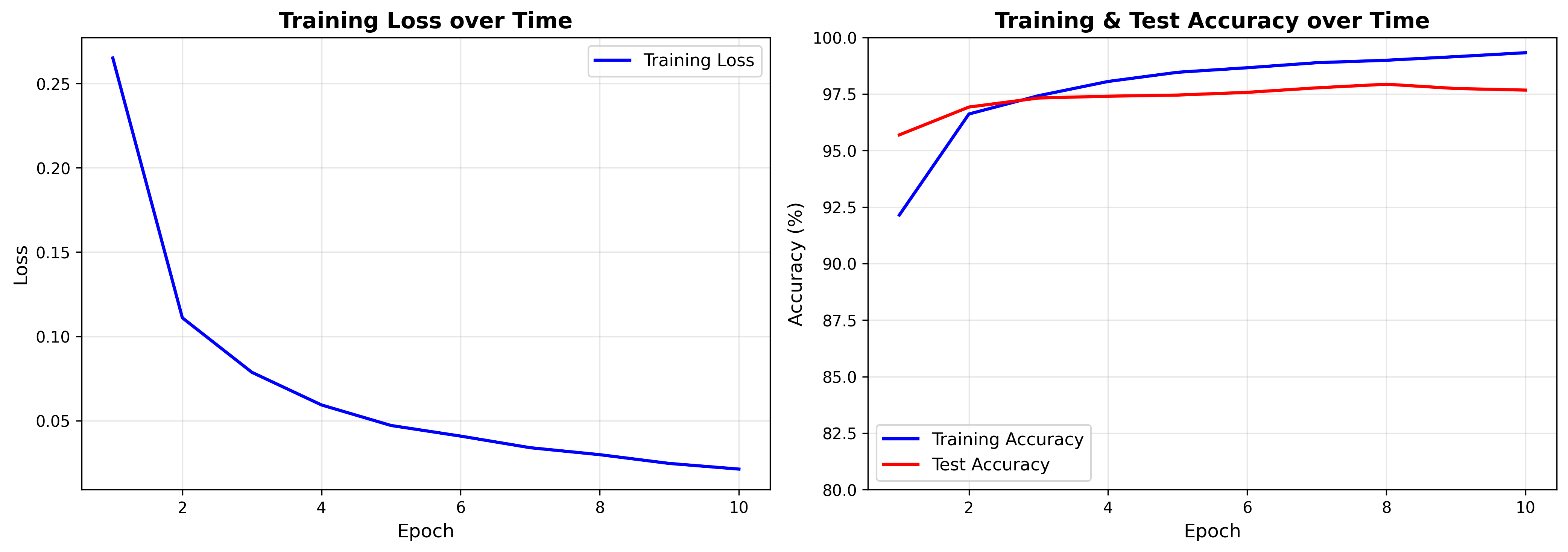
Two plots: training loss falling from 0.27 to 0.02 over ten epochs, and accuracy curves where training accuracy climbs past 99% while test accuracy plateaus near 97.5%. — Ten epochs. Loss falls fast then crawls — and the two accuracy curves separate.

Most tutorials show you the loss curve going down and move on. Look at the right-hand panel instead. Training accuracy climbs past 99% while test accuracy flattens around 97.5% — and actually dips at epoch 9.

That widening gap is the model starting to memorise the training set instead of learning digits. It's mild here, and nothing is broken. But seeing overfitting happen in your own run, in a plot you produced, is worth considerably more than reading the definition. It's also the first thing you'll look for in every model you train after this one.

3 · Open layer 1 — this is the payoff

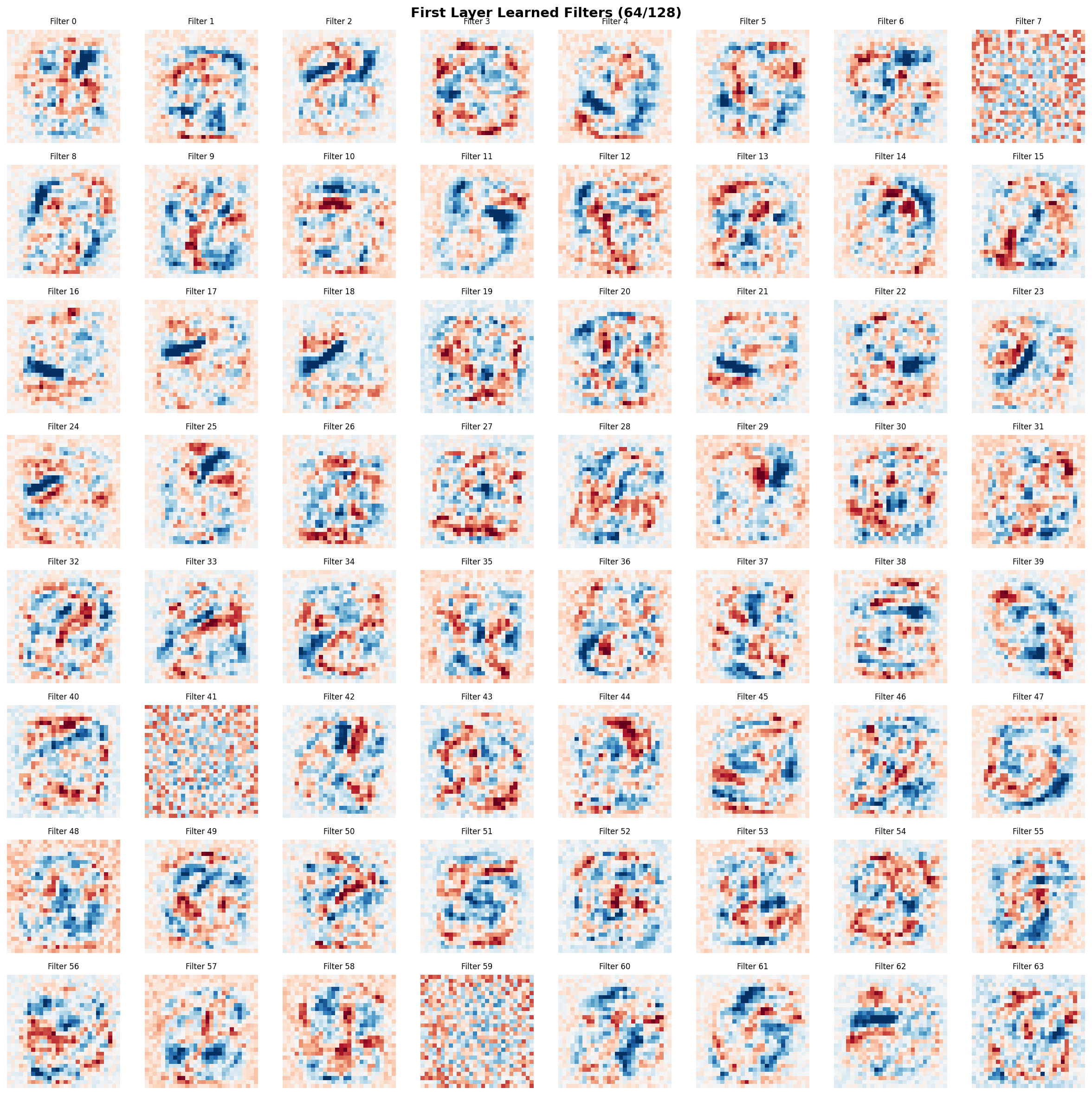
A grid of 64 heatmaps, each showing one first-layer neuron's 784 weights folded back into 28×28. Many show clear diagonal strokes, curves and loops in red and blue; a few remain unstructured noise. — 64 of the first layer's 128 neurons. Each tile is one neuron's 784 weights, folded back into a 28×28 grid — red where it wants ink, blue where it wants blank.

Each neuron in the first layer has exactly 784 weights: one per input pixel. Which means you can fold those weights back into a 28×28 grid and look at them as an image. That picture is what the neuron is looking for.

Nobody designed these. They started as small random numbers. After 82 seconds of gradient descent, you can see diagonal strokes, curved segments, loop detectors — features nobody specified, discovered because they happened to reduce the loss.

Look at tiles 7, 41 and 59, too. They're still noise. Those neurons learned nothing useful, and the network hit 97.5% anyway. That's a real property of these systems worth meeting early: capacity is not evenly used, and a portion of any trained network is effectively dead weight. (On a given input it's not a portion but a majority — I counted the activations for one digit and 60% of this layer sits at exactly zero. That's in the companion piece.)

Layers 2 and 3 are in the repo as well, and they're deliberately less satisfying — by then the network is combining features rather than looking at pixels, so there's no reason for a human-legible picture to survive. The interpretability you get in layer 1 is a gift of being adjacent to the input, not a general property.

4 · Read the mistakes

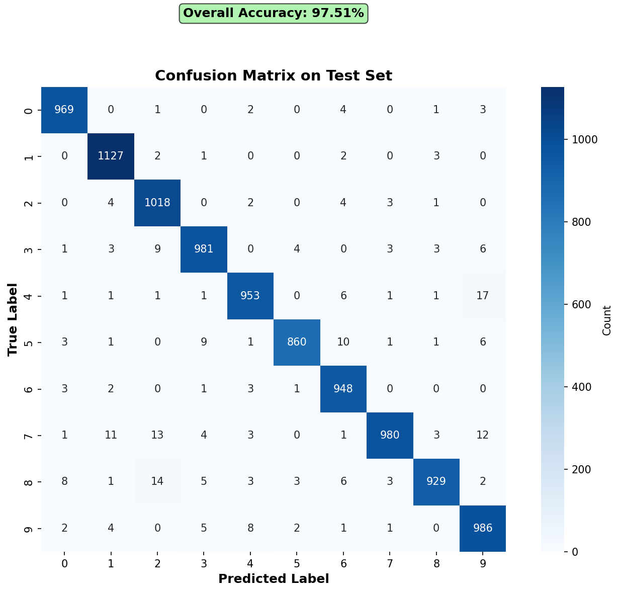
A 10×10 confusion matrix on the MNIST test set with a strong diagonal; the largest off-diagonal counts are 4 predicted as 9 seventeen times, 8 as 2 fourteen times, and 7 as 2 thirteen times. — 249 errors out of 10,000 — and they cluster exactly where you'd expect.

An accuracy number tells you how often the model was wrong. A confusion matrix tells you how it was wrong, which is the part you can act on.

Mine missed 249 of 10,000, and the errors aren't scattered: 4 read as 9 seventeen times, 8 as 2 fourteen times, 7 as 2 thirteen times, 7 as 1 eleven times. Those are the confusions you would make yourself, squinting at bad handwriting. The network converged on human-shaped mistakes without being asked to — and that's a far more interesting result than 97.51%.

Get in the habit here, because it transfers directly: whenever a system gives you an aggregate score, go find the distribution behind it before you believe anything.

The experiment worth running yourself

One question I chased and would recommend: does it matter whether you start the biases at zero or at small random values? Same architecture, same seed, same data, trained twice.

Metric	Random bias	Zero bias
Test accuracy	97.51%	97.67%
Test loss	0.0945	0.0857

Effectively a tie — 0.16% is inside normal variance. But the useful finding is underneath: the two trained models' weights correlate only 0.64 to 0.87 depending on the layer, while agreeing on 97.62% of test predictions. Genuinely different weights, the same competence.

Which kills a tempting intuition — that training discovers the solution. It doesn't. It finds one of enormous numbers of adequate ones, and where it lands depends on where it started. Zero-bias initialisation is still the right default, for reproducibility and clarity rather than accuracy.

Where these figures come from. All four are generated from a single training run that scored 97.51%, by loading that run's weights — they're measurements, not illustrations. The code in the repo now zeroes the biases, so training it today reproduces the 97.67% model instead and your figures will differ slightly from mine. That's correct behaviour, not a bug. I also found that the original filenames were unreliable — a reorganisation script had copied one run's images under two different model names — so the repo's figures are de-duplicated and renamed, and no image there claims to compare two models. The comparison above comes from the numeric dumps.

What this has to do with the models you actually use

This is a 109,386-parameter classifier, not a language model, and I'm not going to pretend the architectures are the same. But three things you can only really learn by watching them happen here hold all the way up.

What's learned is weights. The neuron values you watched light up exist only during a run and vanish when it ends. The weights are the knowledge — and when training stops, they freeze.
Nobody specified the features. No one wrote a stroke detector. It appeared because it reduced loss. Scale that mechanism up and it's why large models are capable and simultaneously hard to explain.
The aggregate hides the behaviour. 97.51% concealed a specific, structured pattern of 4-for-9 errors. Every eval number you'll ever be handed conceals something similar.

If those land, the rest of what every team should know about LLMs stops being abstract — you'll have watched the frozen-weights story happen on your own laptop rather than taken my word for it.

Go do it

Clone mnist-anatomy, run python train.py, wait 82 seconds, then run the visualisation scripts against your own weights. Budget an afternoon rather than a week. The goal isn't to produce a model — the world has enough MNIST classifiers — it's to have looked inside one once, so that every model conversation afterwards has something concrete under it.

And if you want the other half — what the network is actually computing, in the notation, with the backpropagation that produced those filters — that's the same network, written out, drawn by hand.

Then, if you want the same treatment applied to the systems your team actually ships, that's what a Foundations session is for.

← Back to the working notes