The same network, written out

This is the companion to train a network, then look inside it. That piece is empirical: train the thing, then examine what it taught itself. This one answers the other question — what is actually being computed — in the notation, because at some point the notation stops being a barrier and starts being the shortest way to say a simple thing.

The diagrams below are the boards I drew for myself while building it. I'm using them rather than clean typeset maths on purpose: this is what the understanding looked like while it was forming, and the ugly version is more useful than the polished one.

Same network throughout: 784 inputs → 128 → 64 → 10 outputs, 109,386 parameters.

The whole thing on one page

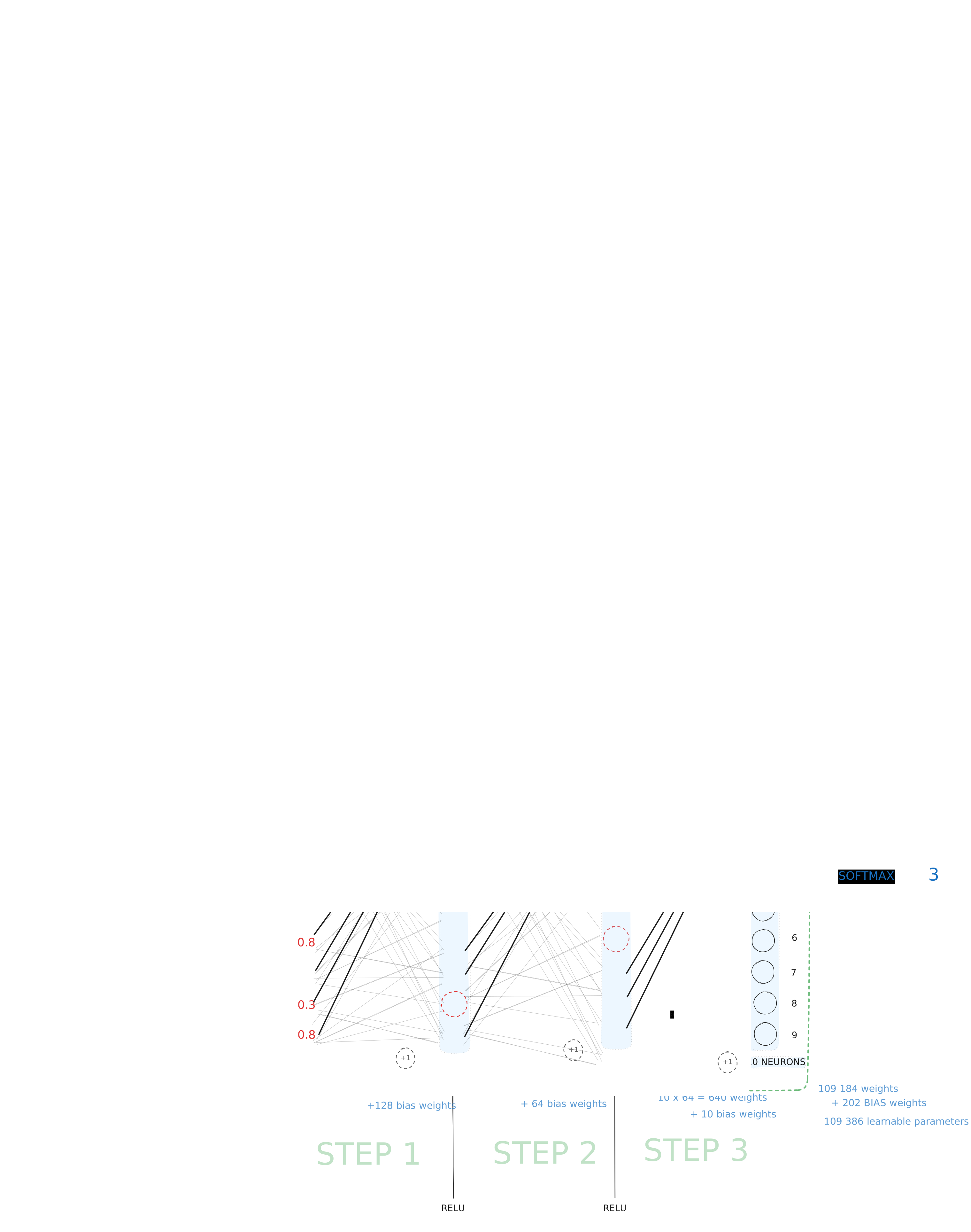
The forward pass end to end: unroll the image, three matrix steps, ReLU twice, softmax once, one digit out. — click to enlarge

Three steps, and each step is the same operation: multiply by a matrix of weights, add a bias, then squash. The image is unrolled first — the 28×28 grid becomes a single column of 784 numbers, and the network never learns that pixel 30 sits directly below pixel 2. Spatial structure is thrown away at the door. It still reaches 97.5%, which tells you how much signal survives even a lossy representation.

One neuron, one pixel at a time

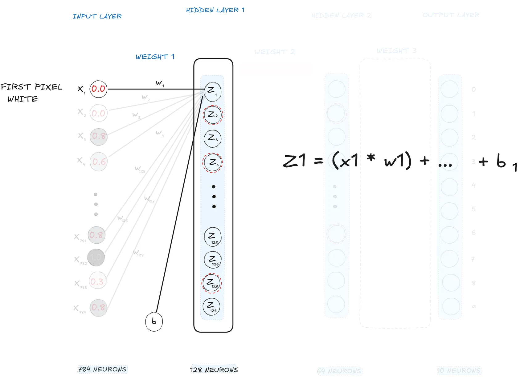
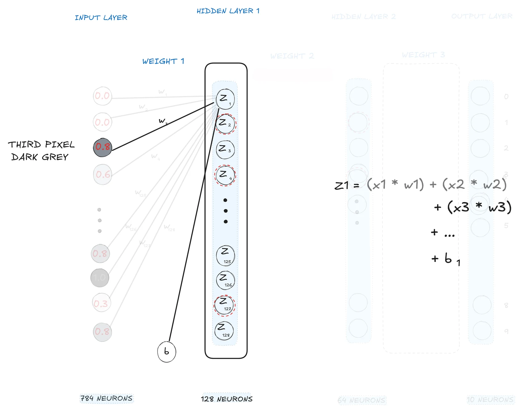
Hand-drawn diagram: the first input pixel with value 0.0 connects through weight w1 to the first neuron of hidden layer 1, with the formula z1 = (x1 * w1) + ... + b1. — First pixel, first weight. The formula has one term so far. — click to enlarge

The same diagram after three pixels: the formula has grown to z1 = (x1*w1) + (x2*w2) + (x3*w3) + ... + b1. — Third pixel. Same neuron, one more term. Repeat 784 times. — click to enlarge

Here is the entire mystery of a neuron, dismantled: take each of the 784 input values, multiply it by that neuron's private weight for that pixel, add all 784 results together, then add one bias. That's the neuron's value.

The weight is how much this neuron cares about that pixel. The bias shifts the threshold at which it gets excited — a strongly negative bias means "only fire if the evidence is overwhelming." Both are numbers that started random and got nudged by training. Nothing else is happening.

128 neurons in this layer, each with its own 784 weights and its own bias. That's 128 × 784 + 128 = 100,480 numbers in the first layer alone — already 92% of the whole model.

Why the notation exists

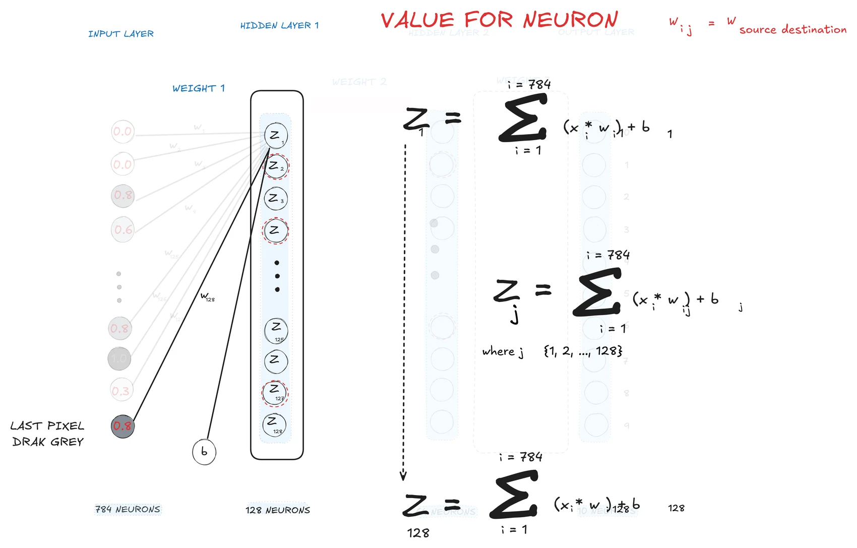
Hand-drawn board titled VALUE FOR NEURON: three stacked formulas showing z1, then the general z_j, then z_128, each as a sum from i=1 to 784 of (x_i times w_ij) plus b_j, with a note that w_ij means w_source,destination. — The same sentence three times: for neuron 1, for any neuron j, for neuron 128. — click to enlarge

Writing out 784 terms is unbearable, so it collapses to one line:

z_j = Σ_i=1..784 (x_i × w_ij) + b_j where j ∈ {1 … 128}

That's it. The sigma is "add up all of these", i walks over the 784 inputs, and j picks which of the 128 neurons you're talking about. The subscript order is the part worth memorising, because it's the part everyone gets backwards: w_ij reads source, then destination — from input i, into neuron j.

With one caveat that will save you an hour later: in the matrix form on the next board, that same weight sits at row j, column i. The matrix is destination × source — which is also the shape PyTorch hands you, since nn.Linear(784, 128).weight has shape [128, 784]. That's precisely why folding one neuron's weights back into a 28×28 image works on a row.

The notation isn't a harder idea. It's the same idea, written short enough to fit on a page.

ReLU — the only nonlinearity between the layers

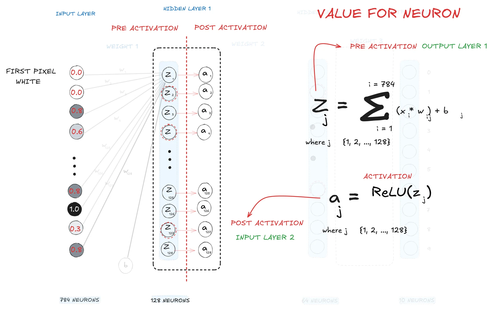
Hand-drawn board showing a red dashed line splitting each neuron into a pre-activation value z and a post-activation value a, with the formula a_j = ReLU(z_j), and a green label noting that post-activation of layer 1 is the input of layer 2. — Every neuron has two values: z before activation, a after. The red line is where one becomes the other. — click to enlarge

The weighted sum gives you z, the pre-activation. Then:

a_j = ReLU(z_j) = max(0, z_j)

Negative becomes zero; positive passes through unchanged. That is the whole function, and it is doing enormous work — because without some nonlinearity between the layers, stacking three matrix multiplications would be mathematically identical to one matrix multiplication. Three layers would collapse into one, and depth would buy you precisely nothing. ReLU is what stops the collapse.

The green annotation on that board is the detail I'd been fuzzy on until I drew it: the post-activation of layer 1 is the input of layer 2. There is no separate object. Layer 2 doesn't receive pixels, it receives 128 activations, and it has no idea they were ever an image.

The real numbers, for one digit

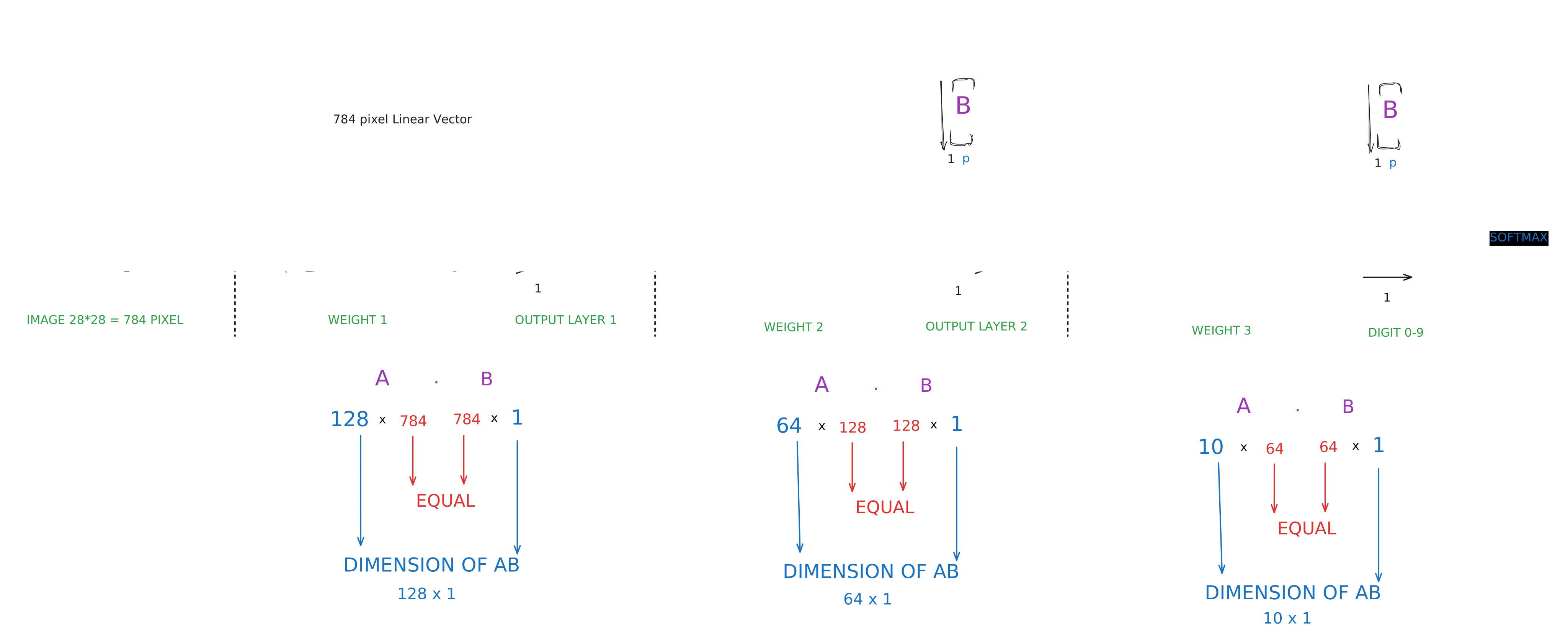
Hand-drawn board showing the three matrix steps and their dimension checks: 128×784 times 784×1 equals 128×1, then 64×128 times 128×1 equals 64×1, then 10×64 times 64×1 equals 10×1, with red EQUAL arrows marking the inner dimensions that have to match. — Three matrix steps, and the shape bookkeeping for each. — click to enlarge

That's a dimension check, and it's the one piece of bookkeeping that catches most beginner bugs: (128 × 784) · (784 × 1) = (128 × 1). The inner numbers must match; the outer numbers are your answer's shape.

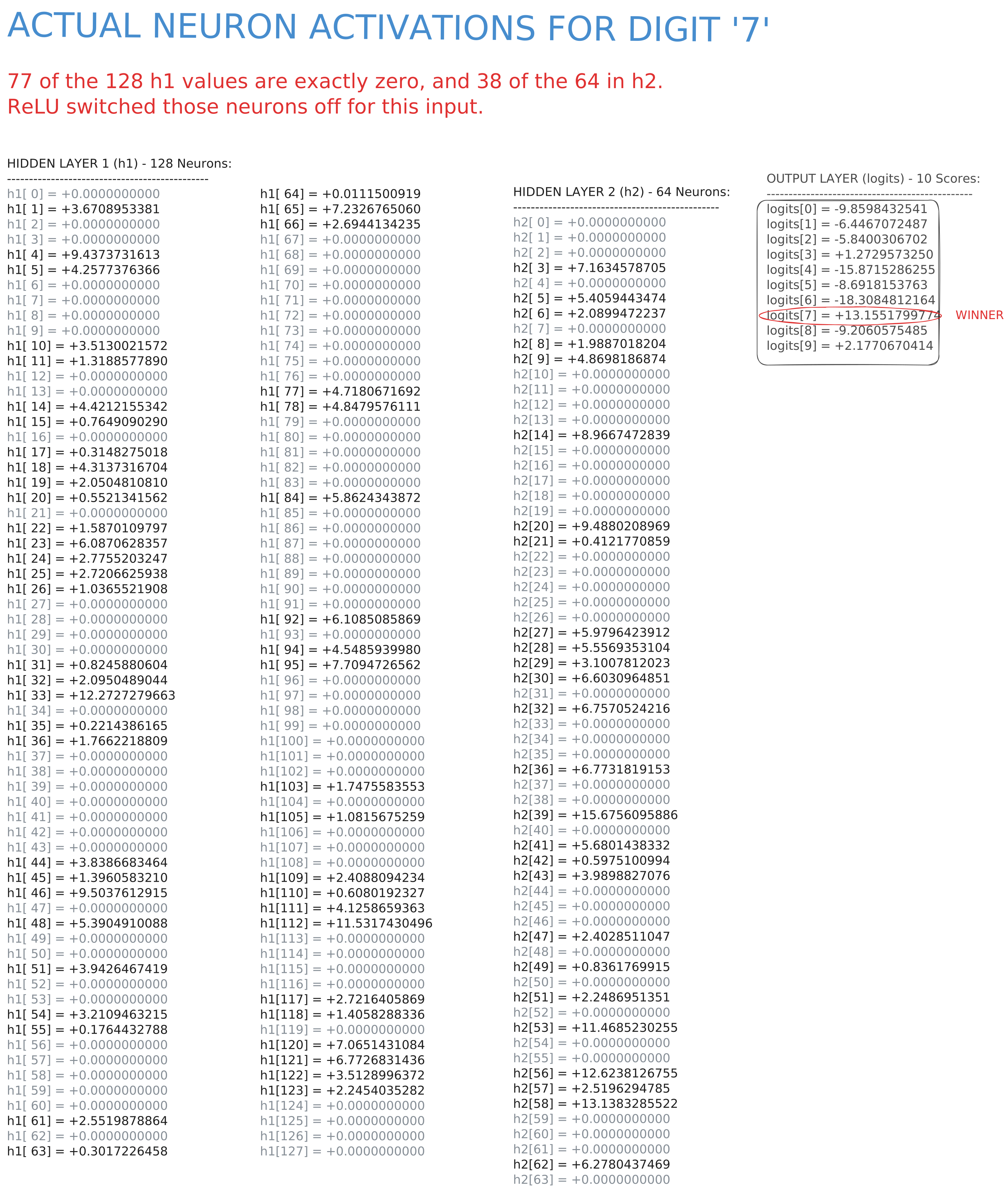
Long printed columns of the actual neuron activation values for a handwritten 7: 128 values for hidden layer 1, 64 for hidden layer 2 and the 10 output logits. Every value that is exactly zero is greyed out, leaving the non-zero minority in black, and logit index 7 is circled in red as the winner. — Measured activations from one real inference. Every greyed row is exactly zero. — click to enlarge

Those are measured values from an actual run. I counted them: of the 128 neurons in hidden layer 1, 77 are exactly zero — 60% of the layer. In layer 2, 38 of 64. That's ReLU, switching most of the network off for this particular input. The greying in that figure is the count made visible: black rows are the neurons that fired.

It's worth keeping this separate from the noisy-looking filters in the first article, because they're different things and it would be easy to conflate them. A filter is a neuron's weights — fixed after training, the same for every input. An activation is what that neuron does on one particular image. A neuron with beautifully structured weights still reads zero whenever its pattern isn't in front of it.

So the silence isn't damage, it's selectivity: for any given digit, most of the network isn't looking. Which is the more interesting claim of the two — a trained network is not a machine where everything fires a bit, it's a large committee of specialists most of whom stay quiet.

Softmax — from scores to something you can read

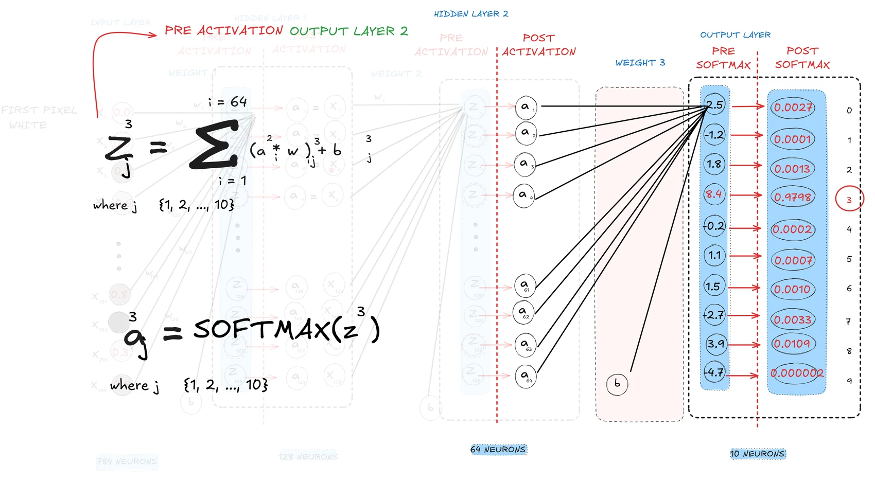
Hand-drawn board showing the ten output neurons with pre-softmax scores such as 2.5, -1.2, 1.8 and 8.4, red arrows converting them into post-softmax probabilities 0.0027, 0.0001, 0.0013 and 0.9798, with the winning digit 3 circled. — Ten raw scores in, ten probabilities out, summing to 1. — click to enlarge

The last layer emits ten unbounded numbers, called logits. They aren't probabilities: they can be negative, they can exceed 1, they don't sum to anything. Softmax fixes that by exponentiating each one and dividing by the total.

One wrinkle if you go reading the code: model.py returns raw logits and contains no softmax. During training the softmax lives inside CrossEntropyLoss instead — same arithmetic, better numerical stability. The board shows the maths; the code puts it one layer down.

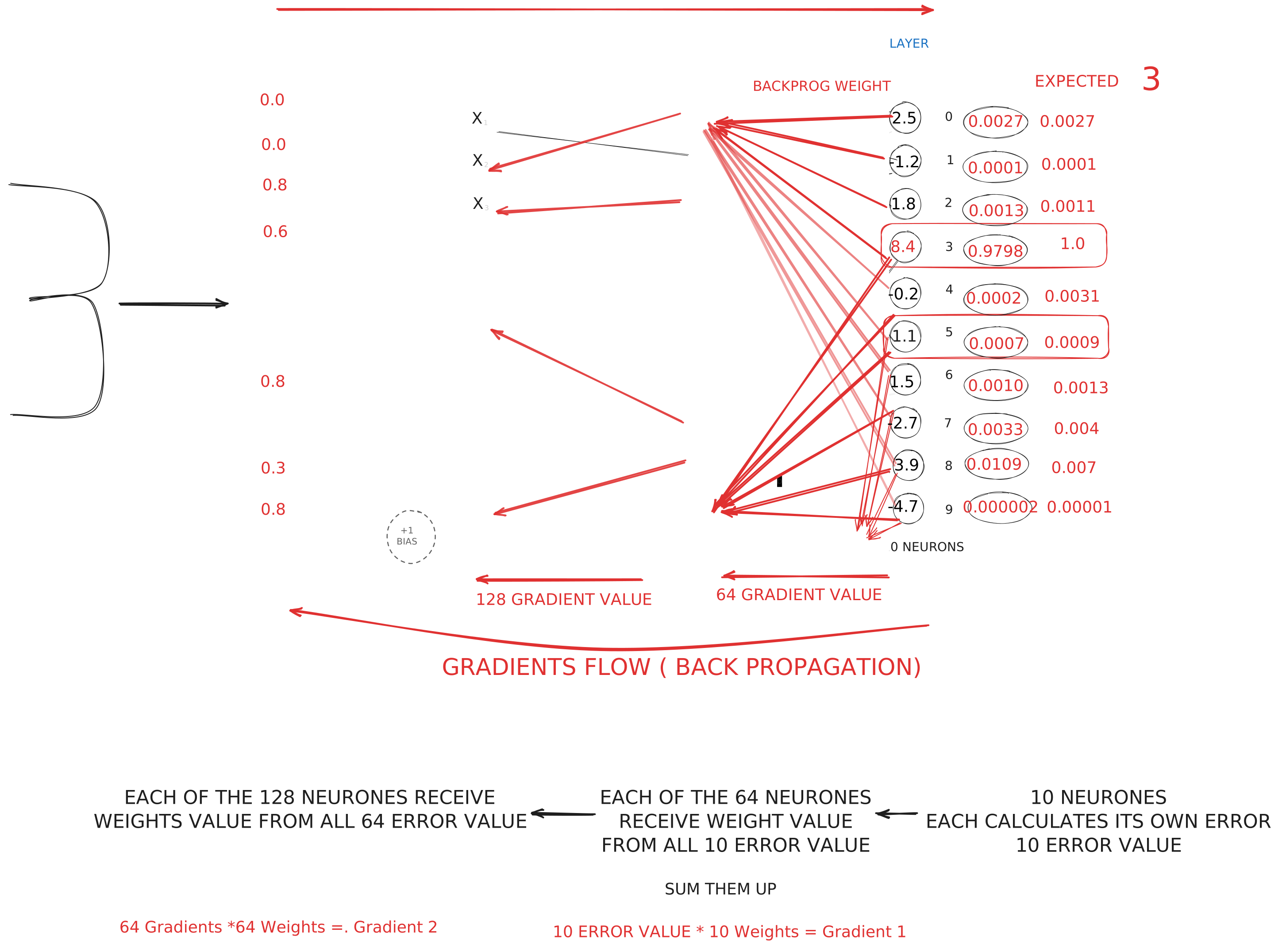
Work the example on that board. The scores are 2.5, −1.2, 1.8, 8.4, −0.2, 1.1, 1.5, 2.7, 3.9, −4.7. Exponentiate: e^8.4 = 4,447 while e^2.5 = 12. The sum of all ten is 4,538 — so digit 3 alone takes 4,447 of it, or 97.98%.

That's the property worth carrying away: the exponential doesn't rank the scores, it amplifies the gap. A lead of 5.9 in raw score becomes a 365× lead in probability. It's also why a model's confidence can look absolute when the underlying scores were merely close-ish — a fact worth remembering the next time something reports 99% certainty.

Where the weights came from

Hand-drawn board on the loss: the expected output compared with what the network actually produced, the definition loss = how far are we from a bullseye perfect shot, then Loss = −ln(probability of the correct class), a drawn curve of −ln(p) exploding as p approaches zero, and the output-layer gradients p−1 for the correct class and p for the wrong ones, worked through with real numbers. — How wrong were we? The loss, and the two gradients that fall out of it. — click to enlarge

Hand-drawn board: a handwritten 3 enters the network, the ten output probabilities are compared with the expected answer, and thick red arrows run backwards from the output layer through the 64 and 128 neuron layers, labelled 64 gradient value and 128 gradient value under the heading gradients flow (back propagation). — The same network, run backwards. Red is the blame travelling from the error to every weight. — click to enlarge

Hand-drawn board: the update rule weight_new = weight_old − (learning_rate × avg_gradient) written large, with learning_rate annotated as an arbitrary constant value, and beneath it the batch mechanics — process in batches of 16 to 128 images, average the gradient every 32, one epoch is 60,000 images once, ten epochs is ten times that. — What actually changes, and how often. — click to enlarge

Everything above describes a network that already knows things. These three boards are where the knowing comes from, and it's the half the first article skips.

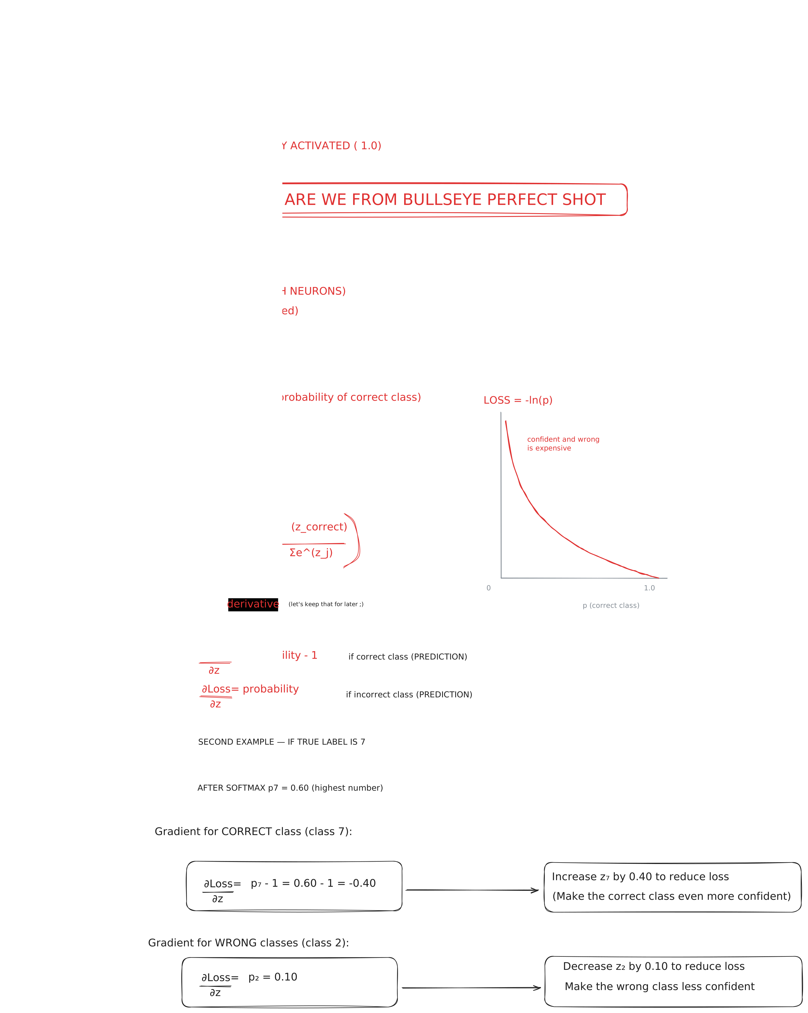
Measure the error. Loss = −ln(probability assigned to the correct class). If the model gave the right answer 0.98, the loss is nearly zero. If it gave it 0.10, the loss is large. The logarithm is what makes confident-and-wrong expensive.
Work out who's to blame. At the output the gradient is beautifully simple: for the correct class it's probability − 1, for every wrong class it's just probability. Predict 0.60 for the right answer and you get −0.40 — a push to raise that score. Then the chain rule carries that blame backwards: 10 error values become gradients for the 64 neurons feeding them, which become gradients for the 128 below.
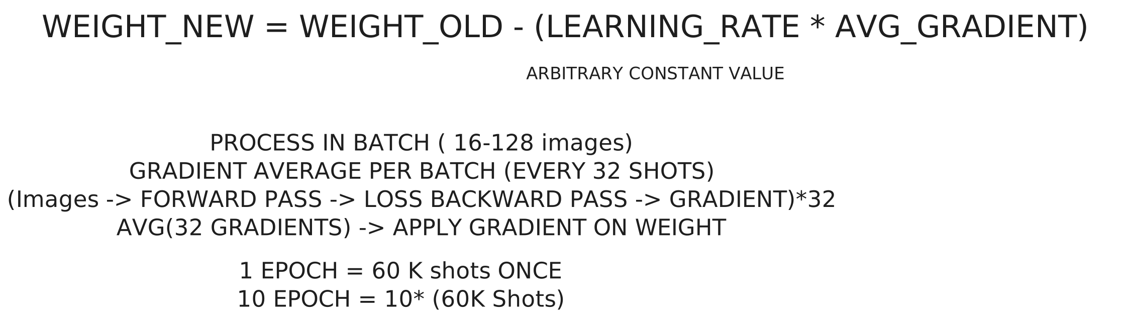
Nudge every weight. weight_new = weight_old − (learning_rate × average_gradient), with the learning rate at 0.001. That's the shape of the idea — though the repo actually uses Adam, which adds per-parameter momentum and adaptive step sizes on top of this rule. The direction is the same; the step size isn't fixed. (0.001 is Adam's default, not a value I tuned.)
Do it in batches, repeatedly. Gradients are averaged over 64 images at a time rather than applied per image, so one weird 7 can't yank the whole model. One epoch is all 60,000 images once; training runs ten of them.

That's 600,000 image presentations and about 9,400 weight updates in 82 seconds — and it is the entire origin of the stroke detectors from the first article. Nobody designed them. They are the accumulated residue of being wrong a lot and adjusting slightly each time.

Why bother with any of this

You do not need this to use a language model, in the same way you don't need engine internals to drive. But there's a specific payoff: once a neuron is visibly just a weighted sum with a threshold, the phrase "the model thinks" stops sounding like a description and starts sounding like the metaphor it is. Every mechanism above is doing arithmetic that a patient person could do by hand — there are only 109,386 numbers.

Be careful how far you carry that, though. The primitive generalises: a language model's neurons are still weighted sums with biases and a nonlinearity, and its final layer still turns scores into probabilities with a softmax. The architecture does not — transformers add attention, embeddings, normalisation and residual connections, none of which are in this network and none of which fall out of it. What you can take upward is the arithmetic and the habits: read the distribution behind the score, expect most of the network to be quiet, remember the weights are frozen. Roughly seven orders of magnitude separate this model from a frontier one, and scale buys behaviour that genuinely doesn't appear here.

Those habits are most of what what every team should know about LLMs is about — written for the models you actually work with, and now with a laptop-sized worked example underneath it.

What's measured and what's a worked example. The activation dump is real output from a genuine inference on a handwritten 7 — I counted the zeros rather than estimating them, and its logits do peak at index 7 with 9 as runner-up, which is exactly the confusion the matrix in the first article predicts. The softmax board is a worked example with clean numbers, chosen to make the arithmetic followable — it's a different digit from the activation dump, and I haven't tied the two together.

If you'd rather build this understanding with your hands than read it, mnist-anatomy has the code, and the first article is where to start. If you want it installed in a team rather than a person, that's a Foundations session.

← Back to the working notes